
RETAINED RESULTS · INDEPENDENTLY CHECKED
Compare the methods.
QPoland 2026 main prize winner · Joint first in the VeloxQ award.
Choose a case and inspect solution quality, feasibility and compute. Every comparison states its input scope.
Choose batches and a feasible production plan.
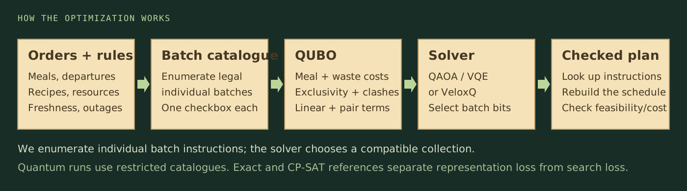
Inputs
Meal orders and departures, recipes and batch yields, resource calendars, worker qualifications and the current kitchen state.
Decisions
Choose quantities, shared allocations, cookers, crew and preparation/cooking/packing/cleaning times on a 10-minute grid.
Constraints and events
Equipment and worker clashes, phase attendance, fresh handovers, mandatory cleaning, committed work, urgent orders, cooker outages and recovery cleaning.
Optimize in this order
Missed complete meals → discarded components → new batches. One lot is 10 portions. The full recorded objective includes R, but current fixtures have R = B, so it only adds to the batch coefficient.
Implemented scope: paired main + side, shared batch yields, independent raw-schedule checker. Money, ingredients, holding/power capacity and interrupted cooking are outside the current model.
Same offered choices. Different search methods.
| Method | Optimum hit | P(optimum) / shot | P(valid) | Best (U,W,B,R) | Median wall |
|---|
Settings were selected on cell/S0/S1, then frozen for S2/S3. Each instance optimizes its own angles. Final sampling uses 4,096 shots. The full-grid reference measures restriction loss; it has more choices than these QUBOs.
Inspect all 400 QAOA runs
| Case / split | Method | Budget / seed | P(optimum) | Best tuple | Wall |
|---|
Test the representation, then compare quality.
Best checked plan out of 140 requested meals, at equal 20,000 steps and 512 replicas. Deleting idle bits also raises valid returns from 17/512 to 512/512. Waste rises from 30 to 60 portions; complete service has lexicographic priority. Same source programs/objective, different sampling matrices.
The new formulation returned 512/512 valid at actual widths 486, 998 and 2,022. CP and same-formulation SA still find better schedules. These are exploratory single-job measurements, not a held-out superiority result.
| Attempt / case | Representation | Solver bits | Replicas × steps | Valid / returned | Best tuple | Backend / full call | Status |
|---|
VeloxQ is a GPU optimization service. Backend runtime excludes preprocessing and transport. Recovered downloads have no successful whole-call time shown. No physical-QPU execution is implied.
Test the ansatz, loss and optimizer.
One-hot Givens rotations plus controlled rotations between coupled blocks; exact CVaR0.1 and adjoint L-BFGS-B. The E5 baseline report reaches the offered-pool optimum in 10/10 S2 seeds and 9/10 S3 seeds. Those per-seed numbers are reported CSV evidence; the five exported cell/S0–S3 schedules have also been independently checked.
| Case / method | Optimum hit | Median P(optimum) | Median P(valid) | Training work | Final shots |
|---|
E6 follow-up: concentrate probability after CVaR
The same coupled two-layer circuit first uses CVaR α = 0.1, then Gibbs η = 100, with exact adjoint gradients and caps of 150 evaluations per stage. The configuration was declared before this follow-up; S2/S3 had already been examined in E5, so these are confirmation cases, not genuinely unseen problems. The E5 baseline above remains unchanged.
| Case / method | Optimum dominates (>50%) | Optimum sampled | Median P(optimum) | Median P(valid) | Adjoint evaluations | Final shots |
|---|
Exact-simulator improvement; the staged method did not reproduce this gain under emulated shot noise. Training work differs from QAOA. The probabilities concern offered-pool optima, not the full scheduling domain. A stopping rule at 99.5% concentration explains the plateau.
| Case | Valid shots | Best tuple | Evaluations | Legacy circuit heuristic |
|---|
Different optimizer, budgets, parameter count and shot count from QAOA: no matched-budget winner is claimed. Archived circuit counts assume two shifts per parameter; that rule is not validated for the controlled gates and CVaR loss and is not a hardware cost estimate. A fresh five-case export includes the cell; all exported schedules are independently checked.
Inspect all VQE experiment rows, including failed runs
E2 three-point NFT uses a single-frequency control assumption that need not hold here. It is an experimental control; primary E5 L-BFGS-B/CVaR results do not use it.
| Case / seed | Configuration | Loss | Optimum sampled | P(optimum) | Evaluations | Status |
|---|
Another cooker, or another worker?
In the best plans found, adding a prep or packing helper serves 110 meals instead of 90. A third cooker serves the same 90. This compares one resource change at a time on the same full physical model.
W1 carries both preparation and packing.
W1 is the only worker qualified for these two jobs. In the retained current-kitchen plan, they occupy 300 of the 320 available minutes.
| One resource change | Meals served | Gain vs current | Discarded portions |
|---|---|---|---|
| Current kitchen | 90 / 140 | +0 | 10 |
| Add a third cooker | 90 / 140 | +0 | 0 |
| Add a prep helper | 110 / 140 | +20 | 10 |
| Add a packing helper | 110 / 140 | +20 | 10 |
Classical CP reference: 240 seconds per run, two solver workers, two seeds; both seeds return the same objective tuples. All displayed plans pass the checker, but none is proved optimal. These runs do not establish that extra equipment can never help. Wages and equipment prices were not supplied, so this is a service-capacity comparison, not a cheapest-hire or ROI result.
Download the full resource study ↗ · Method and all resource variants ↗
Orders, legal programs and their conflicts grow together.
| Workload | Actual width | What the result establishes |
|---|---|---|
| Complete cell | 35 data qubits · 1,045 sector states | Complete on its small declared grid; exact correctness and circuit check. |
| QAOA scenarios | 31–35 data qubits · up to 279,936 sector states | Restricted offered pools; trained sampling quality and measured restriction loss. |
| VeloxQ source pools | 512 / 1,024 / 2,048 bits | Nested restrictions of 18,182 generated local programs. |
| VeloxQ no-idle | 486 / 998 / 2,022 bits | Same program choices with redundant idles removed; feasibility and quality checked. |
The source graph densities are about 28–30%; these matrices are not advertised as sparse. More variables or a reference timeout alone does not establish classical hardness. The QAOA simulator exploits an exact invariant sector. We claim no quantum advantage or extrapolated crossover.
VQE uses the same 31–35-qubit portfolios and exact one-hot-sector simulation. Controlled cross-block gates can entangle blocks; no dense 35-qubit statevector or hardware run is claimed.
Source identities, not invented scores.
The download contains all displayed aggregates, all 400 QAOA run records, all 137 VeloxQ attempts and the retained VQE experiment rows. Large raw amplitudes, packets and archives stay in the repository evidence.
Source paths and SHA-256 hashes
Loading retained benchmark data…